Aakash's Physics Blog

In the first post, we established a general intuition of how forms work and why they may provide a better geometric intuition of what is actually occurring. It was mentioned that these ideas extend the ideas of vector calculus so it seems natural to see how differential operators like gradient, curl, and divergence arise in the context of differential forms. It all comes out of the analysis of the exterior derivative . I will stick to 3 dimensions for now and explain the extension into higher dimensions at the end.

Let’s start by differentiating a 0-form or function . Through chain rule, we know the following.

Multiplying both sides by , we get a nice 1-form which we can “vectorize” like we did in the last post.

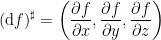
That vector is simply the gradient so “” is equivalent to the gradient operator in some sense for 0-forms.

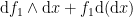
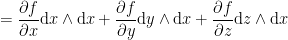
Let’s try to apply this operator to a 1-form instead of a function. We will use the 1-form   where  are functions. Because  is practically a derivative, one can safely assume it is linear.

Let’s just look at the first term. Because  is a 0-form, the first term can be rewritten . If we assume that the  operator follows product rule for derivatives (which to some extent would seem intuitive), the term can be rewritten as follows.

 is just the derivative of a basis vector which is . The first term can be rewritten using our knowledge of gradients and the properties of the wedge product.

At this point, let’s take the Hodge star (it will become clear why soon).

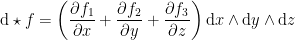
Now, using this calculation, we can generalize it to calculate .

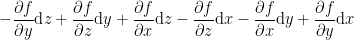
Rearranging and “vectorizing”, we get something very familiar.

This is simply curl and now we can again rewrite familiar vector concepts in the language of forms.

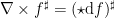
Now what happens with a 2-form? Well, an inconvenience of vector calculus is that it does it does not allow for concepts like 2-forms but we can simply take the Hodge star of a 1-form to acquire one. Assume we have the same , then . Now let’s see what results in. We can calculate the first term with product rule and properties of the wedge product.

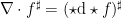
Now, if we generalize this process and solve for the second and third term, we get the following solution.

The Hodge star of this is simply divergence.

There exists one more operator: the Laplacian. This however is easy as it is simply divergence and grad combined or formally the following.

So now we have created all our operators.

This is elegant and shows that all these distinct operators are actually very similar to each other.

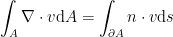
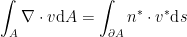
Now, for one more quick step. How is integration defined? For 0-forms, which are just functions, it is the same as usual. For a 1-form, which is basically a vector field, we can integrate across some path which is a familiar concept from vector calculus.

For a two form, which is a planar field, we integrate across some 2-dimensional surface. Here, instead of just using terms like , you would have to use the Jacobian with the parametrization of your surface. Essentially, for any form or vector function , or  because the integral measures the overlap of a form with the manifold being considered. From here, you can build up to higher dimensions so this concept is well-defined.

Now, for the biggest and final step: Stokes Theorem. This is the actual fundamental theorem of calculus.

Let’s start with a few cases.

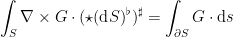
1. Green’s Theorem

This is for two-dimensional vector functions. Classically, it is stated below where  is some vector-valued function.

Let  and  denote the vectors 90 degrees counterclockwise to  and  respectively. Because dotting two rotated vectors doesn’t change the angle in between or the lengths, we know . Then the theorem can be restated.

Because  and  go in the same direction and , we know .

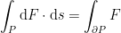
Now to put this in the language of differential forms. First, we substitute the divergence.

Note that I did not use because a 0-form and scalar are not just isomorphic, but equivalent. Knowing this, we see that the left integrand resembles a 2-form.

Now note because the Hodge dual, by definition, represents some sort of orthogonal structure in a space. Remembering how to take integrals for forms, we rewrite the right side of the equation.

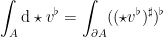
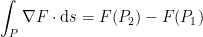
2. Less Generalized Stokes’ Theorem

The theorem is stated below where  is the vector perpendicular to the  element and has a length equal to the area of the  element.

The definition of  should sound immediately familiar when thinking of differential forms. It is simply the Hodge dual of .

The right side is simplified.

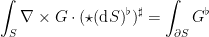
We use our knowledge of curl.

As stated before, dotting the orthogonal version of vectors yields the same results as dotting the vectors themselves.

We once again use our knowledge of integrals of forms.

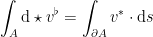
3. Fundamental Theorem of Vector Calculus

There exists the classic fundamental theorem of calculus which is 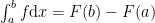. However, there is also the more generalized form that uses gradients and vectors stated below.

and  are the endpoints of path . In some sense, the right side is an integral of the function evaluated only at the endpoints.

We convert the left side using knowledge of forms and path integrals.

Again, was used instead of because it’s a scalar. It’s funny how differential forms makes the originally complex fundamental theorem look so trivial.

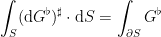
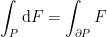
Stokes Theorem

Let us restate all our previous theorems we translated.

They all have the following form where  is some smooth manifold and  is some form.

This is Stokes’ Theorem. In essence, it is saying that by computing small changes within a manifold for some function, we can calculate how much it changes as a whole across it. It is an amazingly powerful yet simple theorem. The most powerful aspect is that it is a general statement that is not limited to any amount of dimensions or space. Note however that I did not, in any sense, prove this. I do not know how to do that but I encourage you to explore it. This is the essence of the differential forms or otherwise known as exterior calculus. There is so much more to explore and much of these last two posts have been hand-wavy anyway so it is worth the time to understand fundamentally what is happening when working through the above equations.

If you want to learn more or see where I started, look at A Quick and Dirty Introduction to Exterior Calculus.